Exponential and logistic growth
If you click on !!! (the menu bar at the top) maple will execute all commands.
You can also enter each command as you go along reading this document. You may enter your own commands at any time and place in this document.
| > |
 |
| > |
 |
Exponential growth
The projection function for logistic growth is
| > |
 |
 |
(1) |
where r>-1 is a constant. When r>0, F(P)>P and the population is increasing; when -1<r<0, F(P)<P and the populationen is decreasing.
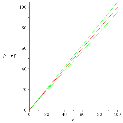
Here are the graphs of the projection functions F(P)=P+rP for r=0.05 (increasing population) and -0.05 (decreasing population) together with the diagonal F(P)=P (constant population)
| > |
![plot([`*`(`+`(1, 0.5e-1), `*`(P)), `*`(`+`(1, -0.5e-1), `*`(P)), P], P = 0 .. 100, labels = [F, F(P)], color = [green, green, red]); 1](images/expo_logi_growth_112.gif) |
The projection function for the increasing population lies above the projection function for the constant population, and the projectione function for the decreasing population lies below it.
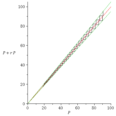
We may illustrate the population dymanics by cobwebs
| > |
![display([cobweb(proc (P) options operator, arrow; `*`(`+`(1, 0.5e-1), `*`(P)) end proc, 20, 32, 0, 100), cobweb(proc (P) options operator, arrow; `*`(.95, `*`(P)) end proc, 90, 32, 0, 100)], labels = ...](images/expo_logi_growth_114.gif)
![display([cobweb(proc (P) options operator, arrow; `*`(`+`(1, 0.5e-1), `*`(P)) end proc, 20, 32, 0, 100), cobweb(proc (P) options operator, arrow; `*`(.95, `*`(P)) end proc, 90, 32, 0, 100)], labels = ...](images/expo_logi_growth_115.gif) |
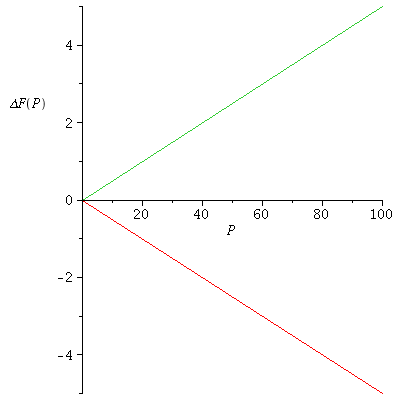
The growth function ΔF(P)=F(P)-P=rP is increasing/decreasing with increasing population density
| > |
![plot([`+`(`-`(`*`(0.5e-1, `*`(P)))), `+`(`*`(0.5e-1, `*`(P)))], P = 0 .. 100, labels = [P, `ΔF`(P)]); 1](images/expo_logi_growth_117.gif) |
The population orbit with P0=2 when r=0.05
| > |
 |
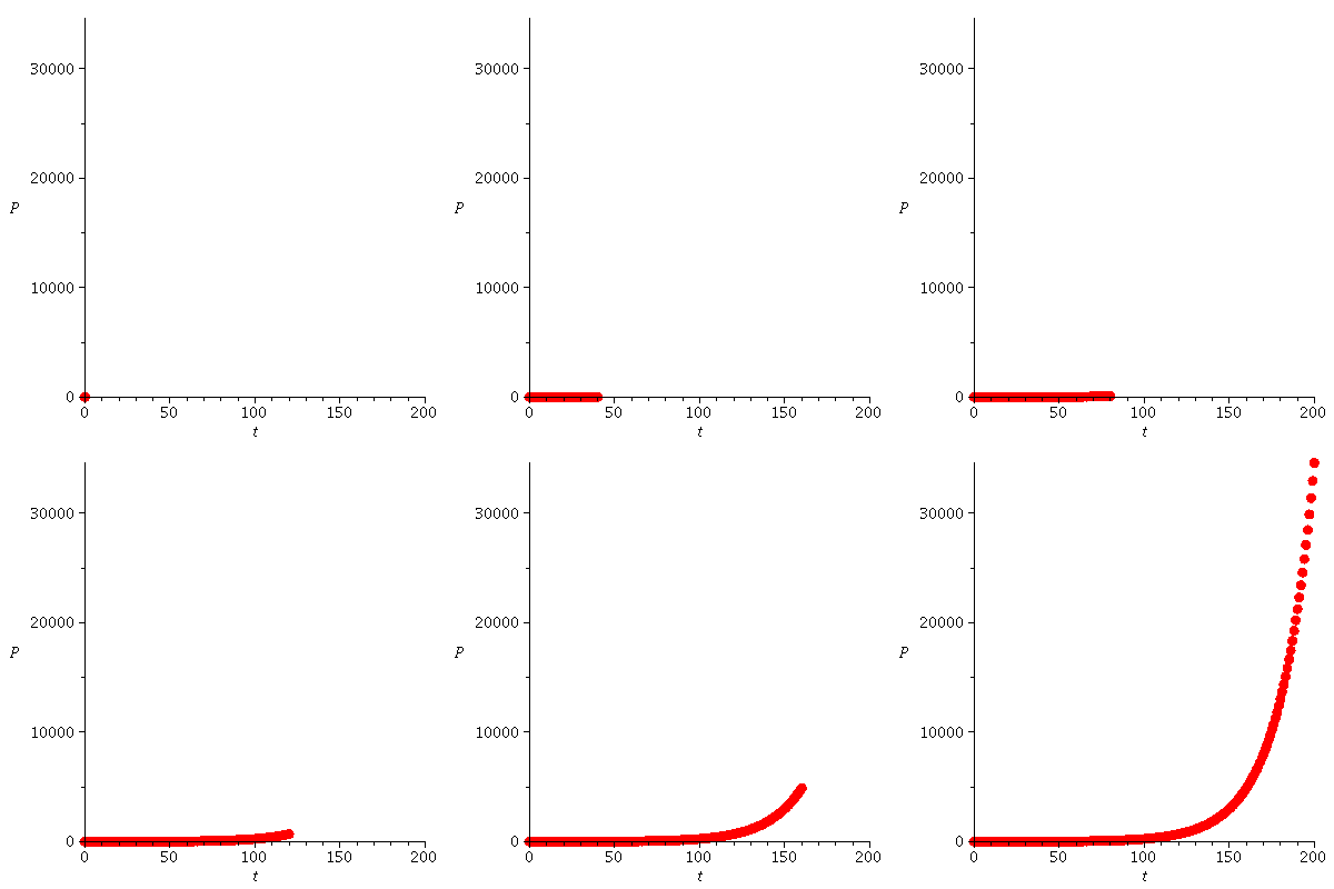
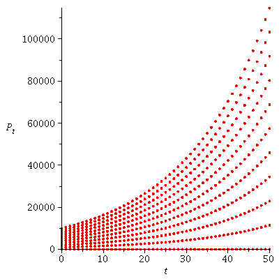
Population orbits with different initial population sizes P0 when r=0.05
| > |
![display(seq(dynplot(proc (P) options operator, arrow; `*`(`+`(1, 0.5e-1), `*`(P)) end proc, `+`(2, `*`(1000, `*`(u))), 50), u = 0 .. 10), labels = [t, P[t]], insequence = false); 1](images/expo_logi_growth_121.gif)
![display(seq(dynplot(proc (P) options operator, arrow; `*`(`+`(1, 0.5e-1), `*`(P)) end proc, `+`(2, `*`(1000, `*`(u))), 50), u = 0 .. 10), labels = [t, P[t]], insequence = false); 1](images/expo_logi_growth_122.gif) |
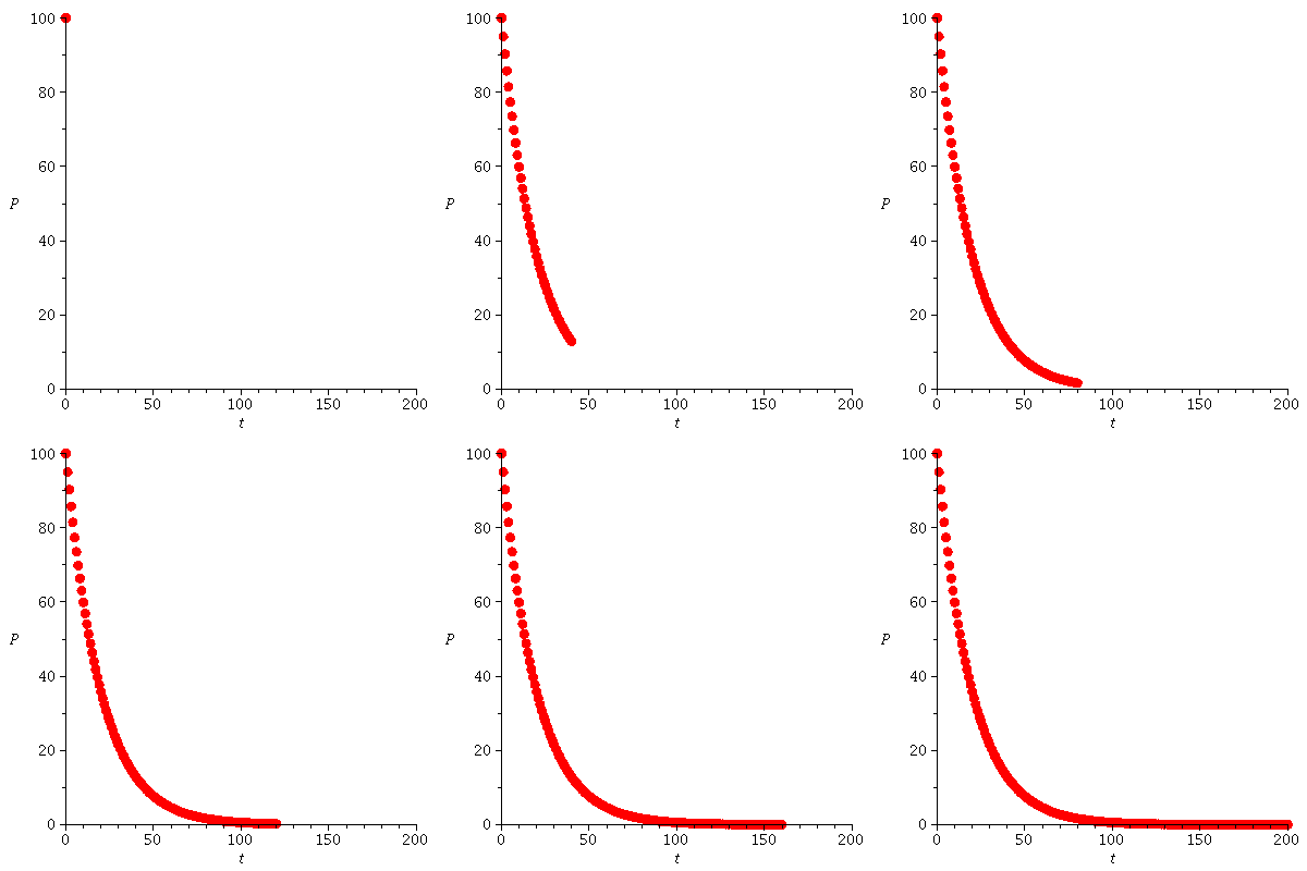
The population orbit with P0=2 when r=-0.05
| > |
 |
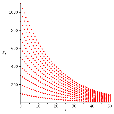
Population orbits with different initial population sizes P0 when r=-0.05
| > |
![display(seq(dynplot(proc (P) options operator, arrow; `*`(.95, `*`(P)) end proc, `+`(100, `*`(100, `*`(u))), 50), u = 0 .. 10), labels = [t, P[t]], insequence = false); 1](images/expo_logi_growth_126.gif)
![display(seq(dynplot(proc (P) options operator, arrow; `*`(.95, `*`(P)) end proc, `+`(100, `*`(100, `*`(u))), 50), u = 0 .. 10), labels = [t, P[t]], insequence = false); 1](images/expo_logi_growth_127.gif) |
Logistic growth
The projection function is
| > |
 |
 |
(2) |
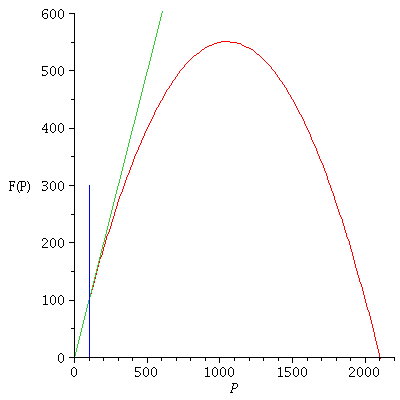
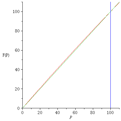
Here is the gaph of the projection function
| > |
 |
 |
(3) |
with r=0.05 and carrying capacity K=100
| > |
![display(plot([(logi(0.5e-1, 100))(P), P], P = 0 .. 2200, y = 0 .. 600, labels = [P,](images/expo_logi_growth_133.gif)
![display(plot([(logi(0.5e-1, 100))(P), P], P = 0 .. 2200, y = 0 .. 600, labels = [P,](images/expo_logi_growth_134.gif) |
The population is increasing, F(P)>P, when 0<P<K, and decreasing, F(P)<P, when P>K.
This may be a little difficult to see on the above graph. It becomes a little more clear if we zoom in on the left part of the graph
| > |
![display(plot([(logi(0.5e-1, 100))(P), P], P = 0 .. 110, y = 0 .. 110, labels = [P,](images/expo_logi_growth_136.gif)
![display(plot([(logi(0.5e-1, 100))(P), P], P = 0 .. 110, y = 0 .. 110, labels = [P,](images/expo_logi_growth_137.gif) |
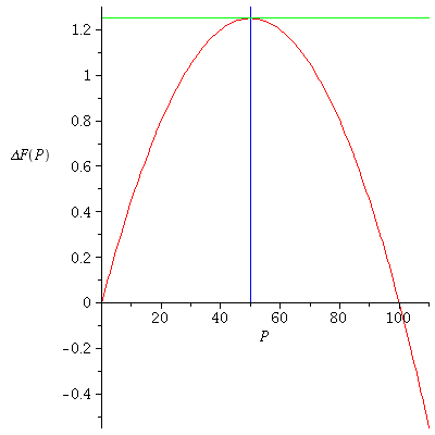
Another way of saying this is that the growth function ΔF(P)=F(P)-P is positive for 0<P<K and negative for P>K.
Here is the graph of the growth function
The growth function ΔF(P)=F(P)-P is maximal when the population densiyt P=K/2 is half of the carrying capacity and negative beyond the carrying capacity K=100.
| > |
![display([plot(`+`((logi(0.5e-1, 100))(P), `-`(P)), P = 0 .. 110, labels = [P, `ΔF`(P)]), implicitplot([P = 50, y = 1.25], P = 0 .. 110, y = 0 .. 1.3, color = [blue, green])]); 1](images/expo_logi_growth_139.gif)
![display([plot(`+`((logi(0.5e-1, 100))(P), `-`(P)), P = 0 .. 110, labels = [P, `ΔF`(P)]), implicitplot([P = 50, y = 1.25], P = 0 .. 110, y = 0 .. 1.3, color = [blue, green])]); 1](images/expo_logi_growth_140.gif) |
The growth function ΔF(P) is maximal when the population density P=K/2 is half of the carrying capacity. The maximal value of the growth function is called Maximal Sustainable Yield or MSY.
The maximal value of the growth function ΔF(P) is achieved when P=K/2 and it is MSY = max ΔF(P) =1/4*K*r. In this particular case, MSY = 1.25.
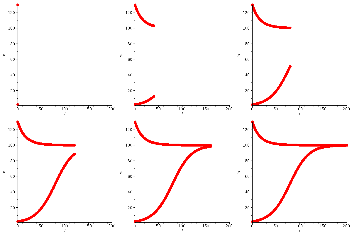
Here are the population orbits at two initial population sizes P0=2 and P0=130
| > |
![display([dynplotfilm(logi(0.5e-1, 100), 2), dynplotfilm(logi(0.5e-1, 100), 130)]); 1](images/expo_logi_growth_142.gif) |
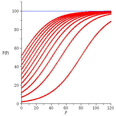
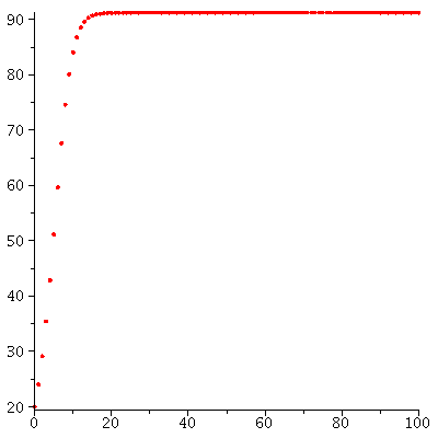
Population orbits with several different initial population sizes P0
| > |

 |
When r<2 there are two equilibria. The equilibrium 0 is unstable and the equilibrium K is stable.
For instance when r=1.8 we can see this by solving the equation F(P)=P for P and computing the derivative F'(P) at the two solutions
| > |
 |
 |
(4) |
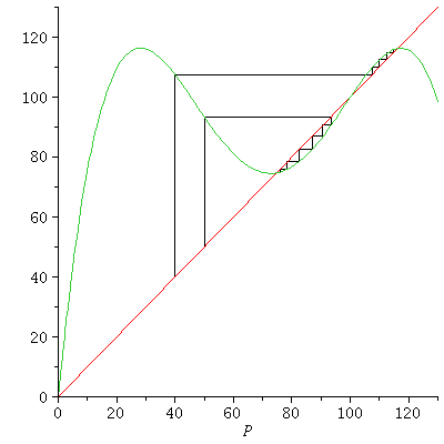
or by drawing cobweb diagrams
| > |
 |
The stable equilibrium determines the long term behaviou becasuse all population orbits (from not too big initial populations) converge to the carrying capacity
| > |
![seq(floor(iterate(logi(1.8, 100), P0, 200)), P0 = [1, 5, 6, 150, 250]); 1](images/expo_logi_growth_151.gif) |
 |
(5) |
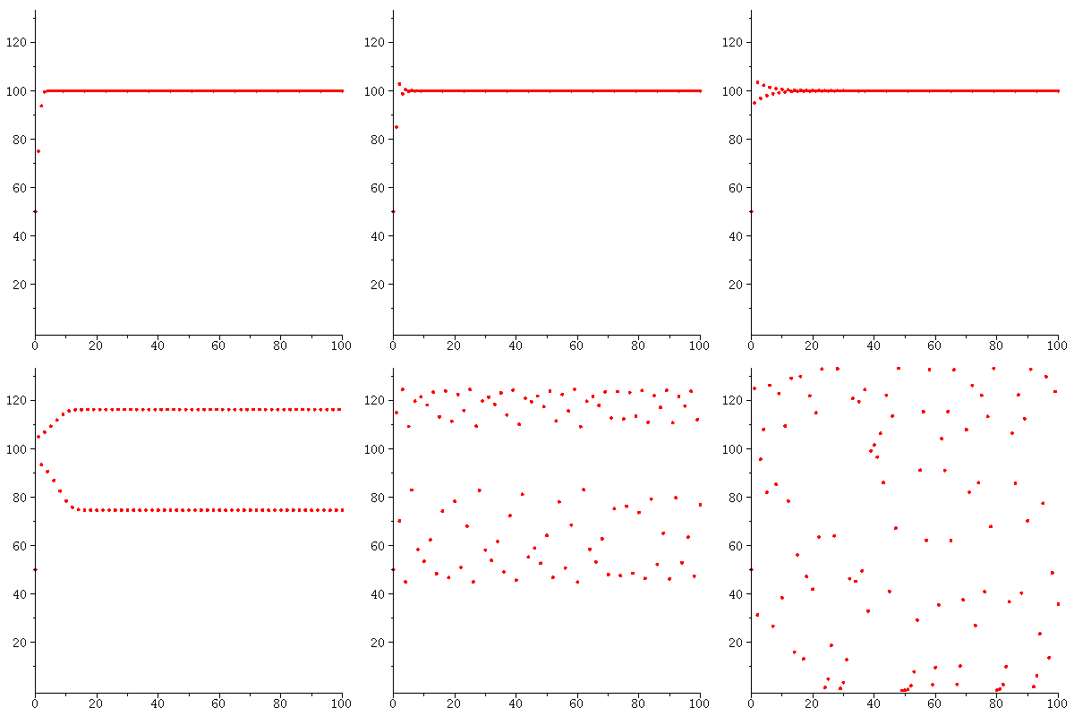
Let us now consider what happens when r>2. Here are four examples with increasing parameter r.
| > |
 |
| > |
 |
| > |
 |
| > |
 |
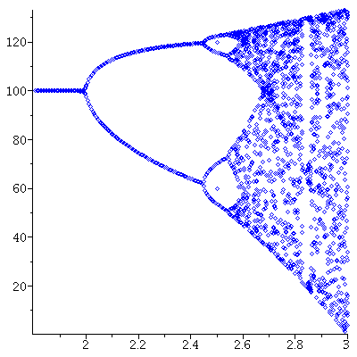
Logistic growth with varying parameter r - stable cycles and chaos emerge
| > |
 |
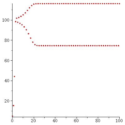
When r is slightly bigger than 2 stable cycles occur.
We look for 2-cycles in logi(2.2,100).
| > |
 |
 |
(6) |
The population dynamics with P0=5 indicates that there is a 2-cycle
| > |
 |
We can find the 2-cycle by solving the equation F(F(P))=P for P. We also compute the derivative (FF)'(P) at each solution to determine stability.
| > |
 |
 |
(7) |
Alternatively, we can use the cobweb diagram for FF
| > |
 |
It looks as if there are stable 2-cycles through 70 and 115 and unstable 2-cycles at 0 and 100.
The stable 2-cycles determine the long term behavior because population orbits will converge to them.
We compute the 100th generation F^100(P0) with four different initial populations
| > |
![seq(iterate(proc (P) options operator, arrow; F(F(P)) end proc, P0, 100), P0 = [40, 50, 80, 120]); 1](images/expo_logi_growth_171.gif) |
 |
(8) |
and check that we indeed have a 2-cycle
| > |
![orbit(F, %[1], 6); 1](images/expo_logi_growth_173.gif) |
 |
(9) |
and that it is stable
| > |
 |
 |
(10) |
| > |
 |
 |
(11) |
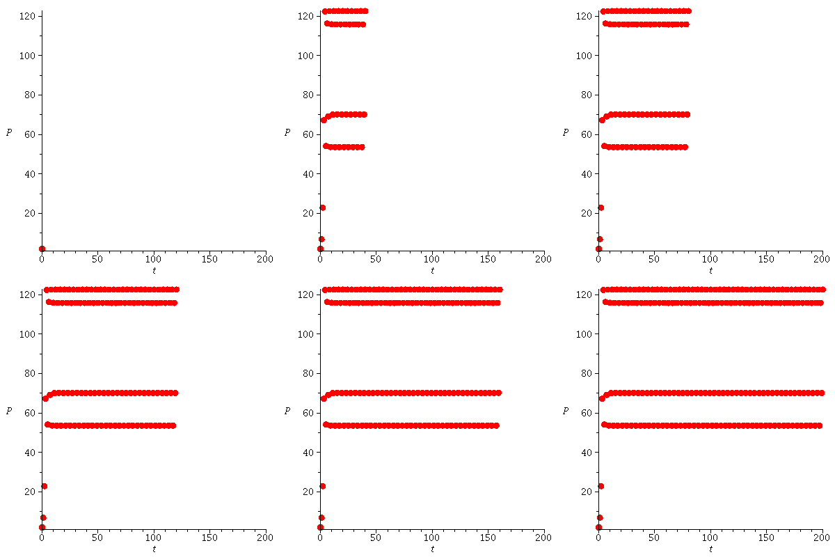
We next look for 4-cycles in logi(2.5,100);
| > |
 |
 |
(12) |
| > |
 |
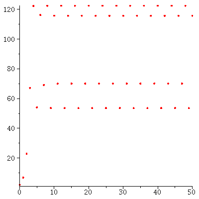
There seems to be a stable 4 cycle near 53.
Any orbit near 53 will converge to it.
| > |
 |
 |
(13) |
We check that this is indeed a 4-cycle
| > |
 |
 |
(14) |
and that it is stable
| > |
 |
 |
(15) |
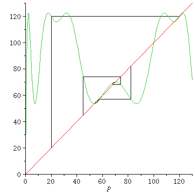
We could also try to compute it directly or use cobweb
| > |
 |
 |
(16) |
| > |

 |
We approximate the stable cycles by orbits
| > |
![seq(iterate(proc (P) options operator, arrow; F(F(F(F(P)))) end proc, P0, 100), P0 = [20, 45, 82, 110]); 1](images/expo_logi_growth_194.gif) |
 |
(17) |
| > |
 |

 |
(18) |
This is the 4-cycle we found before. We have now also found also another cycle, which is a 2-cycle
| > |
 |

 |
(19) |
but it is unstable
| > |
 |
 |
(20) |
| > |
 |
 |
(21) |
The unstability can be illustrated by orbits through points close to P0=20
| > |
![seq(iterate(F, P0, 100), P0 = [19.995, 20, 20.005]); 1](images/expo_logi_growth_206.gif) |
 |
(22) |
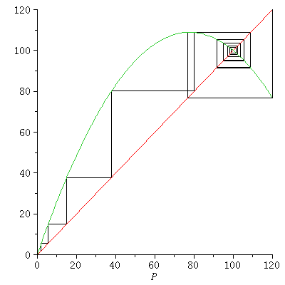
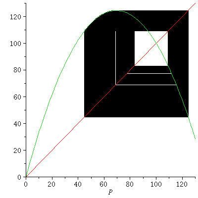
Here is the cobweb diagram with r=2.5:
| > |
 |
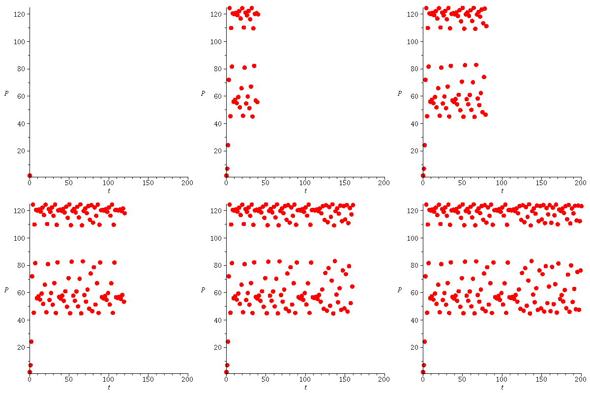
and here is the cobweb diagram with r=2.6:
| > |
 |
The stable orbits are indicated in the bifurcation diagram
| > |
![pointplot([seq(seq([`+`(1.8, `*`(0.5e-2, `*`(i))), orbit(logi(`+`(1.8, `*`(0.5e-2, `*`(i))), 100), 80, 250)[j]], j = 230 .. 250), i = 1 .. 240)], style = point, color = blue); 1](images/expo_logi_growth_212.gif)
![pointplot([seq(seq([`+`(1.8, `*`(0.5e-2, `*`(i))), orbit(logi(`+`(1.8, `*`(0.5e-2, `*`(i))), 100), 80, 250)[j]], j = 230 .. 250), i = 1 .. 240)], style = point, color = blue); 1](images/expo_logi_growth_213.gif) |
Logistic growth with harvest - try to change the harvest
| > |
 |
| > |
 |
Maximal Sustainable Yield MSY
| > |
 |
 |
(23) |
| > |
 |
 |
(24) |
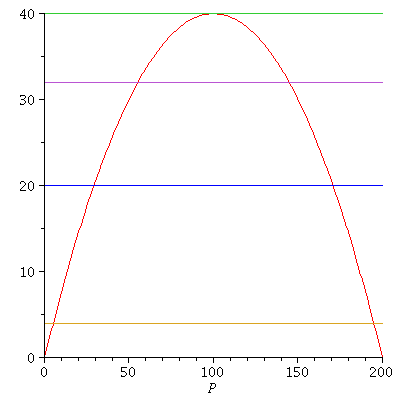
An equilibrium for logistic growth with harvest H is a population size P so that growth ΔF(P) equals harvest, H.
The equilibria can be determined from the intersection points between the graph of the growth function and the horizontal line at level H
| > |
![plot([`+`(F(P), `-`(P)), MSY, `+`(`*`(.1, `*`(MSY))), `+`(`*`(.5, `*`(MSY))), `+`(`*`(.8, `*`(MSY)))], P = 0 .. 200); 1](images/expo_logi_growth_223.gif) |
Let us consider the case where the harvest is
| > |
 |
 |
(25) |
The equilibria are
| > |
 |
 |
(26) |
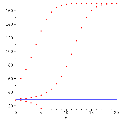
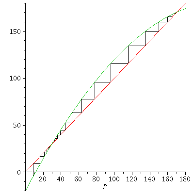
The smallest equilibrium P1=29 is unstable, the biggest P2=170 is stable. This means that if the population size is less than 29, the population will go extinct; if the population is more than 29, it will in the long term stabilize at
population size 170.
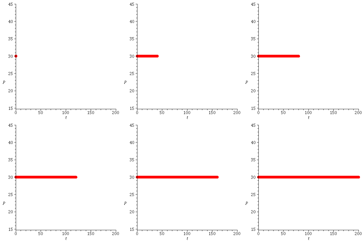
Here are the population orbits from P0=28, P0=30 and P0=50
| > |

 |
We can also see this from the cobweb diagrams from P0=28 and P0=30
| > |
![display([cobweb(proc (P) options operator, arrow; `+`(F(P), `-`(H)) end proc, 28, 7, 0, 180), cobweb(proc (P) options operator, arrow; `+`(F(P), `-`(H)) end proc, 30, 20, 0, 180)]); 1](images/expo_logi_growth_232.gif) |
