Randomized discrete exponential and logistic growth models
What is the definition of a randomized population model? A function F plus a probability distribution X?
| > |
 |
| > |
 |
| > |
 |
| > |
 |
| > |

 |
| > |
![`assign`(orbit, proc (F, P0, T) local j, orb; `assign`(orb, [P0]); for j from 2 to T do `assign`(orb, [op(orb), F(orb[`+`(j, `-`(1))])]) end do; return op(orb) end proc); -1](images/growthdata_7.gif)
![`assign`(orbit, proc (F, P0, T) local j, orb; `assign`(orb, [P0]); for j from 2 to T do `assign`(orb, [op(orb), F(orb[`+`(j, `-`(1))])]) end do; return op(orb) end proc); -1](images/growthdata_8.gif) |
Exponential growth
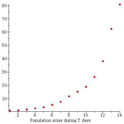
Suppose we have counted the size of a population over T days and obtained the population sizes shown in plot1.
| > |
 |
| > |
 |
| > |
 |
| > |
 |
| > |
![`assign`(P[max], ceil(max(popobs[T]))); -1](images/growthdata_53.gif) |
| > |
![`assign`(plot1, pointplot([seq(`<,>`(j, popobs[j]), j = 1 .. T)], symbol = solidcircle, color = red, symbolsize = 15)); -1](images/growthdata_54.gif)
![`assign`(plot1, pointplot([seq(`<,>`(j, popobs[j]), j = 1 .. T)], symbol = solidcircle, color = red, symbolsize = 15)); -1](images/growthdata_55.gif) |
| > |
 |
Can these data be described reasonably by an exponential growth model?
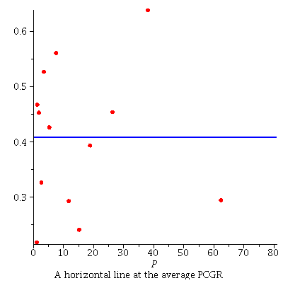
We compute the growth and the per capita growth rate during each of the T-1 time intervals and try to fit it with a horizontal line (the average of the PCGRs).
| > |
![`assign`(GR, seq(`+`(popobs[`+`(j, 1)], `-`(popobs[j])), j = 1 .. `+`(T, `-`(1)))); -1](images/growthdata_58.gif) |
| > |
![`assign`(PCGR, seq(`/`(`*`(GR[j]), `*`(popobs[j])), j = 1 .. `+`(T, `-`(1)))); -1](images/growthdata_59.gif) |
| > |
![`assign`(L, LinearFit([1], popobs[1 .. `+`(T, `-`(1))], [PCGR])); 1](images/growthdata_60.gif) |
](images/growthdata_61.gif) |
(2) |
| > |
![`assign`(r, L[1]); 1](images/growthdata_62.gif) |
 |
(3) |
The estimate is that the observed data can be descibed as discrete exponential growth with per capita growth rate r.
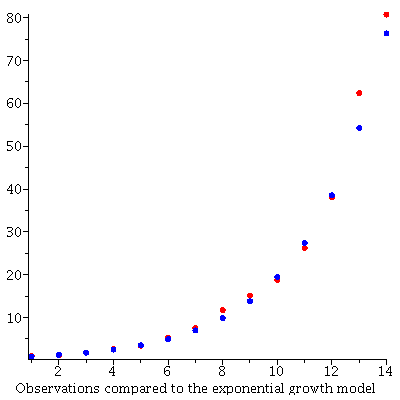
We finally compare the estimated discrete exponential growth model (blue) with the actual observations (red).
| > |
![`assign`(popmodel, orbit(expo(r), `+`(`*`(.9, `*`(popobs[1]))), T)); -1](images/growthdata_68.gif) |
| > |
![`assign`(plot2, pointplot([seq(`<,>`(j, popmodel[j]), j = 1 .. T)], symbol = solidcircle, color = blue, symbolsize = 15)); -1](images/growthdata_69.gif)
![`assign`(plot2, pointplot([seq(`<,>`(j, popmodel[j]), j = 1 .. T)], symbol = solidcircle, color = blue, symbolsize = 15)); -1](images/growthdata_70.gif) |
| > |
![display([plot1, plot2], caption =](images/growthdata_71.gif) |
We didn't estimate the P0 in the model. Try to vary P0 for a better fit.
Logistic growth
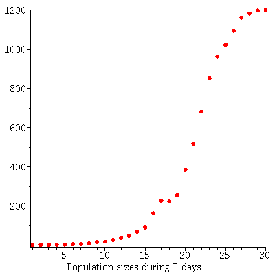
Suppose we have counted the size of a population over T days and obtained the population sizes shown in plot1.
| > |
 |
| > |
 |
| > |
 |
| > |
![`assign`(P[max], ceil(max(popobs[T]))); -1](images/growthdata_76.gif) |
| > |
![`assign`(plot1, pointplot([seq(`<,>`(j, popobs[j]), j = 1 .. T)], symbol = solidcircle, color = red, symbolsize = 15)); -1](images/growthdata_77.gif)
![`assign`(plot1, pointplot([seq(`<,>`(j, popobs[j]), j = 1 .. T)], symbol = solidcircle, color = red, symbolsize = 15)); -1](images/growthdata_78.gif) |
| > |
 |
Can these data be described reasonably by an logistic growth model?
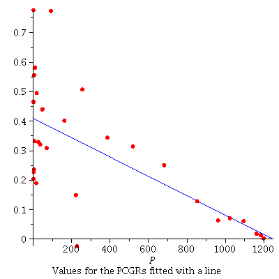
We compute the growth and the per capita growth rate during each of the T-1 time intervals and try to fit it with a line (not necessarily horizontal).
| > |
![`assign`(GR, seq(`+`(popobs[`+`(j, 1)], `-`(popobs[j])), j = 1 .. `+`(T, `-`(1)))); -1](images/growthdata_81.gif) |
| > |
![`assign`(PCGR, seq(`/`(`*`(GR[j]), `*`(popobs[j])), j = 1 .. `+`(T, `-`(1)))); -1](images/growthdata_82.gif) |
| > |
![`assign`(L, LinearFit([1, P], popobs[1 .. `+`(T, `-`(1))], [PCGR], P)); 1](images/growthdata_83.gif) |
 |
(4) |
| > |
 |
| > |
 |
 |
(5) |
| > |
 |
 |
(6) |
The estimate is that the observed data can be descibed as discrete logistic growth with per capita growth rate r and carrying capacity K.
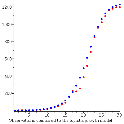
We finally compare the logistic growth model with parameters r and K (blue) with the actual observations (red).
| > |
![`assign`(popmodel, orbit(logi(r, K), `+`(`*`(1.0, `*`(popobs[1]))), T)); -1](images/growthdata_94.gif) |
| > |
![`assign`(plot2, pointplot([seq(`<,>`(j, popmodel[j]), j = 1 .. T)], symbol = solidcircle, color = blue, symbolsize = 15)); -1](images/growthdata_95.gif)
![`assign`(plot2, pointplot([seq(`<,>`(j, popmodel[j]), j = 1 .. T)], symbol = solidcircle, color = blue, symbolsize = 15)); -1](images/growthdata_96.gif) |
| > |
![display([plot1, plot2], caption =](images/growthdata_97.gif) |
The choice of P0 in the model can be important for the fit of these two graphs. We didn't estimate the initial population. Try to modify P0 in the model by varying the factor in front pop_obs[1] in the model.
Stochastic single population models
Exponential growth
| > |
 |
| > |
 |
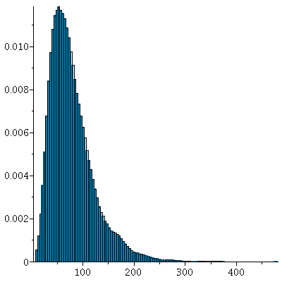
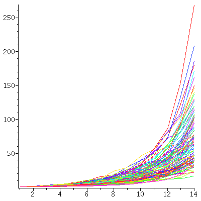
We replicate the experiment 5000 times. and record the final population values.
| > |
![`assign`(runs, [seq(exporand(r, 1, T), j = 1 .. 5000)]); -1](images/growthdata_101.gif) |
| > |
![`assign`(tops, [seq(runs[j][T], j = 1 .. nops(runs))]); -1](images/growthdata_102.gif) |
| > |
 |
![[mean = 79.43496841, standarddeviation = 43.73085118, skewness = 1.658934330, kurtosis = 8.055955291, minimum = 7.914769298, maximum = 481.1628505, cumulativeweight = 5000.]](images/growthdata_104.gif)
![[mean = 79.43496841, standarddeviation = 43.73085118, skewness = 1.658934330, kurtosis = 8.055955291, minimum = 7.914769298, maximum = 481.1628505, cumulativeweight = 5000.]](images/growthdata_105.gif) |
(7) |
| > |
 |
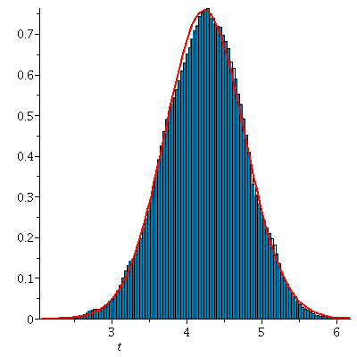
Guess: The logs of the final population sizes is a normal distribution
| > |
![`assign`(logtops, [seq(ln(tops[j]), j = 1 .. nops(runs))]); -1](images/growthdata_108.gif) |
| > |
 |
![[mean = 4.238546730, standarddeviation = .5261152434, skewness = -0.7975874542e-1, kurtosis = 2.983301519, minimum = 2.068730545, maximum = 6.176205779, cumulativeweight = 5000.]](images/growthdata_110.gif)
![[mean = 4.238546730, standarddeviation = .5261152434, skewness = -0.7975874542e-1, kurtosis = 2.983301519, minimum = 2.068730545, maximum = 6.176205779, cumulativeweight = 5000.]](images/growthdata_111.gif) |
(8) |
| > |

 |
| > |
 |
| > |
![display([Hlog, pl1]); 1](images/growthdata_115.gif) |
Here is a graph of the first runs of the model
| > |
![`assign`(S, [seq([seq(runs[k][t], k = 1 .. `+`(`*`(`/`(1, 50), `*`(nops(runs)))))], t = 1 .. T)]); -1](images/growthdata_117.gif) |
| > |
 |
Logistic growth
| > |
 |
| > |
 |
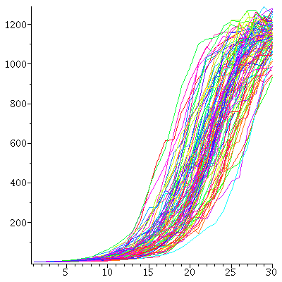
We replicate the experiment 5000 times. and record the final population values.
| > |
![`assign`(runs, [seq(logirand(r, K, 1, T), j = 1 .. 5000)]); -1](images/growthdata_122.gif) |
| > |
![`assign`(tops, [seq(runs[j][T], j = 1 .. nops(runs))]); -1](images/growthdata_123.gif) |
| > |
 |
![[mean = 1140.958515, standarddeviation = 87.66163470, skewness = -1.358680079, kurtosis = 7.292290075, minimum = 437.2256243, maximum = 1393.714210, cumulativeweight = 5000.]](images/growthdata_125.gif)
![[mean = 1140.958515, standarddeviation = 87.66163470, skewness = -1.358680079, kurtosis = 7.292290075, minimum = 437.2256243, maximum = 1393.714210, cumulativeweight = 5000.]](images/growthdata_126.gif) |
(9) |
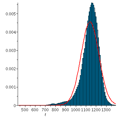
Guess 1: The final population sizes follow a normal distribution (as the final population sizes are close to the carrying capacity when r is not too big)
| > |

 |
| > |
 |
| > |
![display([H, pl1]); 1](images/growthdata_130.gif) |
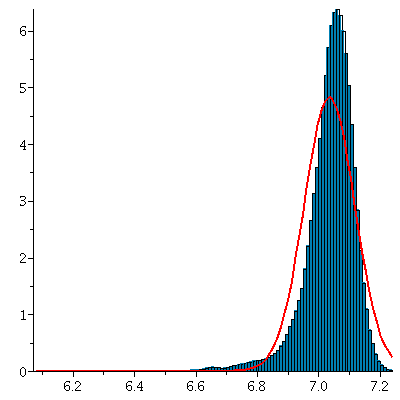
Guess 2:The log(final popsizes) follow normal distribution
| > |
![`assign`(logtops, [seq(ln(tops[j]), j = 1 .. nops(runs))]); -1](images/growthdata_132.gif) |
| > |
 |
![[mean = 7.036379195, standarddeviation = 0.8277494682e-1, skewness = -2.095428191, kurtosis = 13.00661230, minimum = 6.080449365, maximum = 7.239727556, cumulativeweight = 5000.]](images/growthdata_134.gif)
![[mean = 7.036379195, standarddeviation = 0.8277494682e-1, skewness = -2.095428191, kurtosis = 13.00661230, minimum = 6.080449365, maximum = 7.239727556, cumulativeweight = 5000.]](images/growthdata_135.gif) |
(10) |
| > |

 |
| > |
 |
| > |
![display([Hlog, pl1]); 1](images/growthdata_139.gif) |
None of the guesses look good
Here is a graph of the first runs of the model
| > |
![`assign`(S, [seq([seq(runs[k][t], k = 1 .. `+`(`*`(`/`(1, 50), `*`(nops(runs)))))], t = 1 .. T)]); -1](images/growthdata_141.gif) |
| > |
 |





































![[1, 1.218296384, 1.787718988, 2.597335872, 3.445250543, 5.260351783, 7.503081341, 11.71192258, 15.14186888, 18.79296858, 26.19041587, 38.07821000, 62.38167275, 80.74863187]](images/growthdata_50.gif)
![[1, 1.218296384, 1.787718988, 2.597335872, 3.445250543, 5.260351783, 7.503081341, 11.71192258, 15.14186888, 18.79296858, 26.19041587, 38.07821000, 62.38167275, 80.74863187]](images/growthdata_51.gif)
![[1, 1.218296384, 1.787718988, 2.597335872, 3.445250543, 5.260351783, 7.503081341, 11.71192258, 15.14186888, 18.79296858, 26.19041587, 38.07821000, 62.38167275, 80.74863187]](images/growthdata_52.gif)
![display([plot(r, P = 0 .. P[max], color = blue, thickness = 2), pointplot([seq(`<,>`(popobs[j], PCGR[j]), j = 1 .. `+`(T, `-`(1)))], symbol = solidcircle, color = red, symbolsize = 15)], caption =](images/growthdata_64.gif)
![display([plot(r, P = 0 .. P[max], color = blue, thickness = 2), pointplot([seq(`<,>`(popobs[j], PCGR[j]), j = 1 .. `+`(T, `-`(1)))], symbol = solidcircle, color = red, symbolsize = 15)], caption =](images/growthdata_65.gif)
![display([plot(r, P = 0 .. P[max], color = blue, thickness = 2), pointplot([seq(`<,>`(popobs[j], PCGR[j]), j = 1 .. `+`(T, `-`(1)))], symbol = solidcircle, color = red, symbolsize = 15)], caption =](images/growthdata_66.gif)
![display([plot(L(P), P = 0 .. max(P[max], K), color = blue), pointplot([seq(`<,>`(popobs[j], PCGR[j]), j = 1 .. `+`(T, `-`(1)))], symbol = solidcircle, color = red, symbolsize = 15)], caption =](images/growthdata_90.gif)
![display([plot(L(P), P = 0 .. max(P[max], K), color = blue), pointplot([seq(`<,>`(popobs[j], PCGR[j]), j = 1 .. `+`(T, `-`(1)))], symbol = solidcircle, color = red, symbolsize = 15)], caption =](images/growthdata_91.gif)
![display([plot(L(P), P = 0 .. max(P[max], K), color = blue), pointplot([seq(`<,>`(popobs[j], PCGR[j]), j = 1 .. `+`(T, `-`(1)))], symbol = solidcircle, color = red, symbolsize = 15)], caption =](images/growthdata_92.gif)