Spatially realistic Levins metapopulation models after Hanski and Ovaskainen
| > |
 |
We consider the metapopulation model (9) from the paper by Hanski and Ovaskainen 2001.
Construction of the landscape matrix and computation of metapopulation capacity
We consider n patches supporting metapopulations. The n carrying capacities are listed in the 1 x n matrix A. The distances between patches are listed in the symmetric n x n matrix B. The constant exp(α), here denoted a, describes the "average migration distance".
Based on the input A (carrying capacities), B (distances), and a (average migration distance) we construct a "landscape matrix":
| > |
 `(i, j), `*`(A[1, i], `*`(A[1, j], `*`(`^`(a,..." align="center" border="0"> `(i, j), `*`(A[1, i], `*`(A[1, j], `*`(`^`(a,..." align="center" border="0">
 `(i, j), `*`(A[1, i], `*`(A[1, j], `*`(`^`(a,..." align="center" border="0"> `(i, j), `*`(A[1, i], `*`(A[1, j], `*`(`^`(a,..." align="center" border="0"> |
This symmetric matrix has an orthonormal basis of eigenvectors with real eigenvalues.
If a=1, the distance between any two patches is 1.
The metapopulation capacity of this landscape is computed by
| > |

 |
Here is an example with 3 patches , all of carrying capacity 1, and with distances 2,1,4 between them:
| > |
![`assign`(A, Matrix(1, 3, [1, 1, 1])); 1](images/hanski_6.gif) |
 |
(1) |
| > |
 |
 |
(2) |
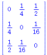
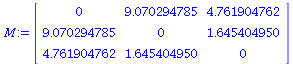
The landscape matrix is
| > |
 |
 |
(3) |
and the metapopulation capacity of this landscape is
| > |
 |
 |
(4) |
Compute the equilibrium
Attached to model (9) is a number δ defined as e/c where e describes the extension rate and c the colonization rate.
Hanski and Ovaskainen show that model (9) achieves a nontrivial equilibrium iff δ<λ(M) where λ(M) stands for the leading eigenvalue of the landspace matrix M.
The next program has as input the landscape matrix M and the number δ. The output is this nontrivial equilibrium. 
| > |
 `(seq(p[i], i = 1 .. d)))[j], `*`..." align="center" border="0"> `(seq(p[i], i = 1 .. d)))[j], `*`..." align="center" border="0">
 `(seq(p[i], i = 1 .. d)))[j], `*`..." align="center" border="0"> `(seq(p[i], i = 1 .. d)))[j], `*`..." align="center" border="0">
 `(seq(p[i], i = 1 .. d)))[j], `*`..." align="center" border="0"> `(seq(p[i], i = 1 .. d)))[j], `*`..." align="center" border="0"> |
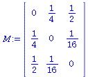
With landscape matrix
| > |
 |
 |
(5) |
there are nontrivial equilibria as long as 
| > |
 |
 |
(6) |
We compute the equilibrium when 
| > |
 |
![[[p[1] = 0., p[2] = 0., p[3] = 0.], [p[1] = .1610695864, p[2] = 0.9000625261e-1, p[3] = .1469908506]]](images/hanski_25.gif) |
(7) |
The interpretation of this is (?) that eg patch number 1 will be occupied to 0.16 of its carrying capacity.
A smaller δ means that the patches are more filled up. For instance for δ=0.2:
| > |
 |
![[[p[1] = .6956425850, p[2] = .517916648, p[3] = .6552859803]]](images/hanski_27.gif) |
(8) |
we see that patch number 1 is occupied to 0.69 of its carrying capacity.
There should not exist an equilibrium when δ=0.59. This is confirmed by the program:
| > |
 |
Compute the relative values of the patches
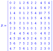
This procedure computes the metapopulation capacity and the relative value of each patch. The input is the carrying capacity of all patches, the distances between patches, and the avreage migration distance a.
An example with 3 patches (A and B are as above)
| > |
 |
| > |
 |
An example with 10 patches
| > |
![`assign`(A, Matrix(1, 10, [1, 2, 3, 4, 5, 6, 1, 2, 3, 4])); 1](images/hanski_46.gif) |
 |
(12) |
 |
(13) |
| > |
 |
The model.
# p[i] is P[i]/K[i] where P[i] is the population and K[i] the carrying capacity at ith patch in this metapopulation model
| > |
![`assign`(orbit, proc (F, P0, T) local j, orb; `assign`(orb, [P0]); for j from 2 to T do `assign`(orb, [op(orb), F(orb[`+`(j, `-`(1))])]) end do; return orb end proc); -1](images/hanski_76.gif)
![`assign`(orbit, proc (F, P0, T) local j, orb; `assign`(orb, [P0]); for j from 2 to T do `assign`(orb, [op(orb), F(orb[`+`(j, `-`(1))])]) end do; return orb end proc); -1](images/hanski_77.gif) |
An example with three patches
| > |
![`assign`(A, Matrix(1, 3, [5, 2, 1])); 1](images/hanski_86.gif) |
 |
(15) |
| > |
 |
 |
(16) |
| > |
 |
 |
(17) |
| > |
 |
 |
(18) |
| > |
 |
![[[p[1] = 0., p[2] = 0., p[3] = 0.], [p[1] = .7601776592, p[2] = .7249883455, p[3] = .616014401]]](images/hanski_95.gif) |
(19) |
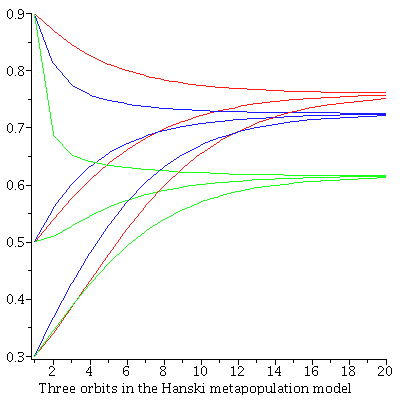
Here is an orbit that converges to the equilibrium
| > |
![orbit(hanski(A, B, 1.05, .1, .3), `<,>`(.2, .3, .2), 100)[100]; 1](images/hanski_96.gif) |
](images/hanski_97.gif) |
(20) |
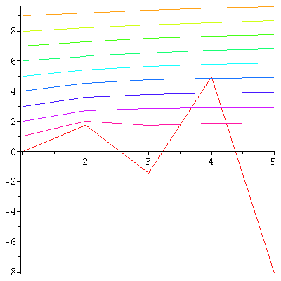
Here are three orbits in the relative form of the model
An example with 10 patches
| > |
![`assign`(A, Matrix(1, 10, [1, 2, 3, 4, 5, 6, 7, 8, 9, 10])); -1](images/hanski_107.gif) |
| > |
 |
 |
(21) |
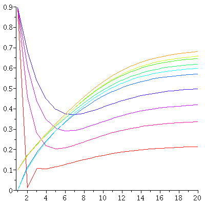
Orbits in the relative form of the model
| > |
 |
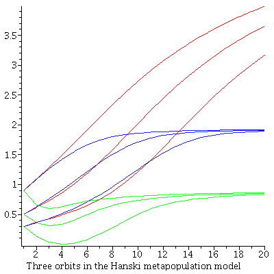
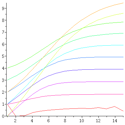
Orbits in the absolute form of the model
| > |
 |
Are the limits just the carrying capacities? If so, what is this model good for?
| > |
 |
Here are some test runs of the program equi (only of mathematical interest)
Example 1
| > |
![`assign`(m3, Matrix(3, 3, [0, 1, 2, 1, 0, 3, 2, 3, 0])); 1](images/hanski_122.gif) |
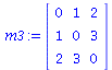 |
(22) |
This is a symmetric matrix with eigenvalues
| > |
 |
](images/hanski_125.gif) |
(23) |
| > |
 |
![[[p[1] = .6991651394, p[2] = .7534021944, p[3] = .7853403267]]](images/hanski_127.gif) |
(24) |
| > |
 |
![[[p[1] = .5676919075, p[2] = .6318589311, p[3] = .6689443743]]](images/hanski_129.gif) |
(25) |
| > |
 |
This seems to be a bug in Maple because
| > |
 |
![[[p[1] = .4454710267, p[2] = .5108974036, p[3] = .5478831809]]](images/hanski_132.gif) |
(27) |
| > |
 |
![[[p[1] = .3308463116, p[2] = .3901921239, p[3] = .4229351864]]](images/hanski_134.gif) |
(28) |
| > |
 |
![[[p[1] = .2225865491, p[2] = .2694980444, p[3] = .2947262123]]](images/hanski_136.gif) |
(29) |
| > |
 |
![[[p[1] = 0.2160958925e-1, p[2] = 0.2745991009e-1, p[3] = 0.3044380018e-1]]](images/hanski_138.gif) |
(30) |
| > |
 |
![[[p[1] = 0.2490829553e-2, p[2] = 0.3179660428e-2, p[3] = 0.3529120804e-2]]](images/hanski_140.gif) |
(31) |
| > |
 |
Example 2
| > |
![`assign`(m4, Matrix(3, 3, [0, 1, 1, 1, 0, 1, 1, 1, 0])); 1](images/hanski_142.gif) |
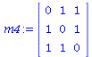 |
(33) |
This is a symmetric matrix with eigenvalues
| > |
 |
](images/hanski_145.gif) |
(34) |
| > |
 |
![[[p[1] = .5000000000, p[2] = .5000000000, p[3] = .5000000000]]](images/hanski_147.gif) |
(35) |
| > |
 |
![[[p[1] = 0.5000000000e-1, p[2] = 0.5000000000e-1, p[3] = 0.5000000000e-1]]](images/hanski_149.gif) |
(36) |
| > |
 |
Example 3
| > |
![`assign`(m5, Matrix(3, 3, [1, 2, 3, 0, 1, 0, 1, 1, 0])); 1](images/hanski_151.gif) |
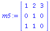 |
(38) |
This matrix is not symmetric. The eigenvalues are
| > |
 |
](images/hanski_154.gif) |
(39) |
and the leading eigenvalue is
| > |
 |
![[[p[1] = 0., p[2] = 0., p[3] = 0.], [p[1] = .845207880, p[2] = 0., p[3] = .6283102355], [p[1] = .8912603423, p[2] = .5000000000, p[3] = .7356260326]]](images/hanski_157.gif)
![[[p[1] = 0., p[2] = 0., p[3] = 0.], [p[1] = .845207880, p[2] = 0., p[3] = .6283102355], [p[1] = .8912603423, p[2] = .5000000000, p[3] = .7356260326]]](images/hanski_158.gif) |
(40) |
| > |
 |
![[[p[1] = 0, p[2] = 0, p[3] = 0], [p[1] = `+`(`-`(2), `*`(`^`(7, `/`(1, 2)))), p[2] = 0, p[3] = `+`(`/`(5, 6), `-`(`*`(`/`(1, 6), `*`(`^`(7, `/`(1, 2))))))]]](images/hanski_160.gif) |
(41) |
| > |
 |
![[[p[1] = 0., p[2] = 0., p[3] = 0.], [p[1] = .646184304, p[2] = 0., p[3] = .3927732002], [p[1] = .6467120554, p[2] = 0.1000000000e-2, p[3] = .3933365602]]](images/hanski_162.gif)
![[[p[1] = 0., p[2] = 0., p[3] = 0.], [p[1] = .646184304, p[2] = 0., p[3] = .3927732002], [p[1] = .6467120554, p[2] = 0.1000000000e-2, p[3] = .3933365602]]](images/hanski_163.gif) |
(42) |
| > |
 |
![[[p[1] = 0., p[2] = 0., p[3] = 0.], [p[1] = .645794616, p[2] = 0., p[3] = .3924146130], [p[1] = .6458476131, p[2] = 0.1000000000e-3, p[3] = .3924710940]]](images/hanski_165.gif)
![[[p[1] = 0., p[2] = 0., p[3] = 0.], [p[1] = .645794616, p[2] = 0., p[3] = .3924146130], [p[1] = .6458476131, p[2] = 0.1000000000e-3, p[3] = .3924710940]]](images/hanski_166.gif) |
(43) |
| > |
 |
![[[p[1] = 0., p[2] = 0., p[3] = 0.], [p[1] = .601851217, p[2] = 0., p[3] = .3536450256]]](images/hanski_168.gif) |
(44) |
| > |
 |
![[[p[1] = 0., p[2] = 0., p[3] = 0.], [p[1] = 0.1514804e-2, p[2] = 0., p[3] = 0.6581769e-3]]](images/hanski_170.gif) |
(45) |
Example 4
| > |
![`assign`(m6, Matrix(3, 3, [0, 1, 3, 1, 0, 2, 1, 4, 0])); 1](images/hanski_171.gif) |
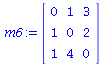 |
(46) |
| > |
 |
](images/hanski_174.gif) |
(47) |
| > |
 |
 |
(48) |
| > |
 |
![[[p[1] = 0., p[2] = 0., p[3] = 0.], [p[1] = .503763461, p[2] = .4389418528, p[3] = .5304647250]]](images/hanski_178.gif) |
(49) |
| > |
 |
![[[p[1] = 0., p[2] = 0., p[3] = 0.], [p[1] = 0.1163434426e-1, p[2] = 0.9176983415e-2, p[3] = 0.1224368977e-1]]](images/hanski_180.gif) |
(50) |
| > |
 |
![[[p[1] = 0, p[2] = 0, p[3] = 0]]](images/hanski_182.gif) |
(51) |