The Lotka-Volterra model
If you click on !!! (the menu bar at the top) maple will execute all commands.
You can also enter each command as you go along reading this document. You may enter your own commands at any time and place in this document.
Procedures
The Lotka-Volterra model is a 2-population model for prey-predator interaction.
In this model, the prey population (P_1) in itself follows logistic growth with parameters (K,r)=(1, 1.3) and the predator population (P_2) in itself follows exponential growth (actually, decay) with parameter u=1-0.7 = 0.3. In addition, there is an interaction term proportional to the number of prey times the number of predators. This interaction has a negative influence on the prey population and a positive influence on the predator population.
The projection function is
| > |
 |
The P_1-isoclines
| > |
![solve((LV(K, r, s, u, v))(P)[1] = P[1], [P[1], P[2]]); 1](images/lotka_volterra_139.gif) |
![[[P[1] = 0, P[2] = P[2]], [P[1] = `/`(`*`(K, `*`(`+`(r, `-`(`*`(s, `*`(P[2])))))), `*`(r)), P[2] = P[2]]]](images/lotka_volterra_140.gif) |
(1) |
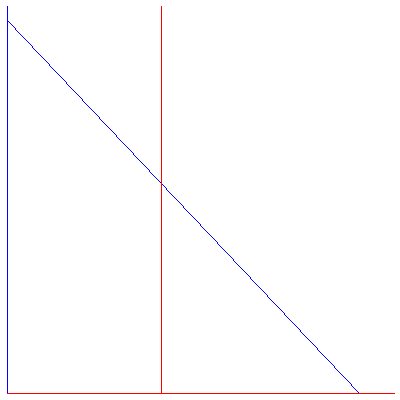
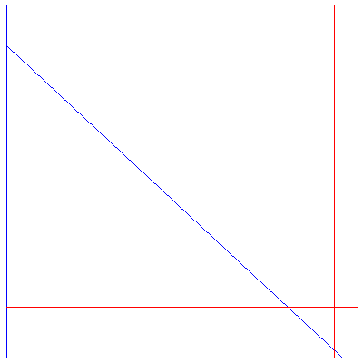
are the vertical line P_1=0 and the line through (K,0) and r/s.
The P_2 isoclines
| > |
![solve((LV(K, r, s, u, v))(P)[2] = P[2], [P[1], P[2]]); 1](images/lotka_volterra_141.gif) |
![[[P[1] = P[1], P[2] = 0], [P[1] = `/`(`*`(u), `*`(v)), P[2] = P[2]]]](images/lotka_volterra_142.gif) |
(2) |
are the horizontal line P_2=0 and the vertical line P_1=u/v.
There are two cases to consider
Case 1: K>u/v There is an equilibrium in the first quadrant
| > |
![implicitplot([P[1] = 0, VectorCalculus:-`+`(P[1], VectorCalculus:-`*`(VectorCalculus:-`*`(.5, `/`(1.3)), P[2])) = 1, P[1] = VectorCalculus:-`*`(.7, `/`(1.6)), P[2] = 0], P[1] = 0 .. 1.1, P[2] = 0 .. 2...](images/lotka_volterra_143.gif)
![implicitplot([P[1] = 0, VectorCalculus:-`+`(P[1], VectorCalculus:-`*`(VectorCalculus:-`*`(.5, `/`(1.3)), P[2])) = 1, P[1] = VectorCalculus:-`*`(.7, `/`(1.6)), P[2] = 0], P[1] = 0 .. 1.1, P[2] = 0 .. 2...](images/lotka_volterra_144.gif) |
Case 2: K<u/v There is no equilibrium in the first quadrant
| > |
![implicitplot([P[1] = 0, VectorCalculus:-`+`(VectorCalculus:-`*`(`/`(1.2), P[1]), VectorCalculus:-`*`(VectorCalculus:-`*`(.5, `/`(1.3)), P[2])) = 1, P[1] = VectorCalculus:-`*`(.7, `/`(.5)), P[2] = 0], ...](images/lotka_volterra_146.gif)
![implicitplot([P[1] = 0, VectorCalculus:-`+`(VectorCalculus:-`*`(`/`(1.2), P[1]), VectorCalculus:-`*`(VectorCalculus:-`*`(.5, `/`(1.3)), P[2])) = 1, P[1] = VectorCalculus:-`*`(.7, `/`(.5)), P[2] = 0], ...](images/lotka_volterra_147.gif) |
We shall not consider this case anymore as it is not biologically interesting (and mathematically there is no reason to distinguish between the two cases).
Equilibria in the LV-model: The equilibria are the crossings between a P_1- and a P_2-isocline
| > |
 |
The Jacobians at the equilibria are
| > |
![simplify(subs({P[1] = 0, P[2] = 0}, Jacobian((LV(K, r, s, u, v))(P), [P[1], P[2]]))); 1](images/lotka_volterra_156.gif) |
 |
(4) |
| > |
![simplify(subs({P[1] = K, P[2] = 0}, Jacobian((LV(K, r, s, u, v))(P), [P[1], P[2]]))); 1](images/lotka_volterra_158.gif) |
 |
(5) |
| > |
![simplify(subs({P[1] = VectorCalculus:-`*`(u, `/`(1, `*`(v))), P[2] = VectorCalculus:-`*`(VectorCalculus:-`*`(r, VectorCalculus:-`+`(VectorCalculus:-`*`(K, v), VectorCalculus:-`-`(u))), `/`(1, `*`(Vect...](images/lotka_volterra_160.gif) |
 |
(6) |
Case 1
Here is an example of a typical projection function with an equilibrium in the first quadrant.
The parameters of the projection function are (K,r,s,u,v)=(1, 1.3, 0.5, 0.7, 1.6).
| > |
 |

 |
(7) |
The equilibria for this particular model are
| > |
 |
The equilibrium in the first quadrant is stable and the equilibria on the axes are saddle points.
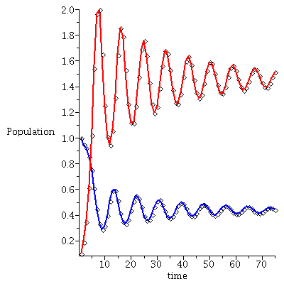
Here is the time plot for prey (blue) and predator (red) over 75 generations with initial population vector <1, 0.1>
| > |
 |
Note that the population vector exhibits a damped oscillation towards an equilibrium.
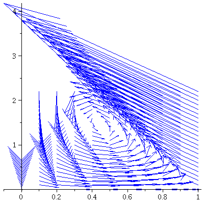
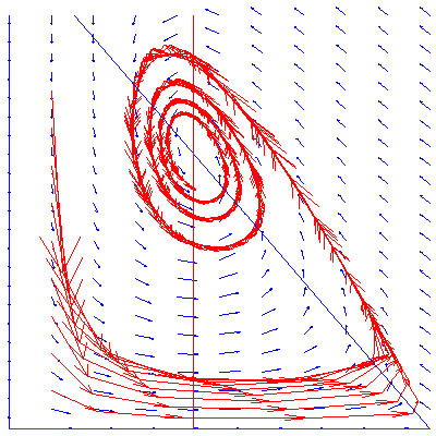
We may also visualize the model by drawing a vector from each point (P_1,P_2) in the plane to F(P_1,P_2). This is the growth field.
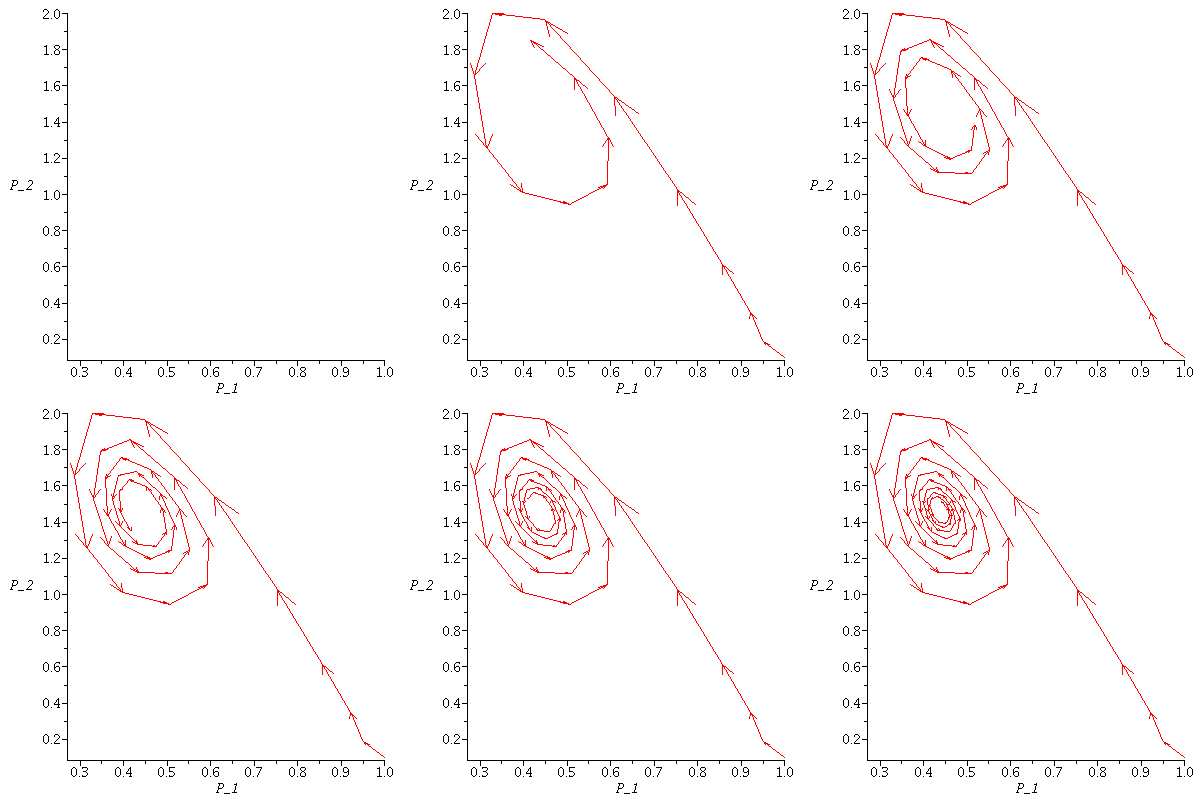
The population orbit starting at a particular point is found by jumping from arrowhead to next arrowhead.
| > |
 |
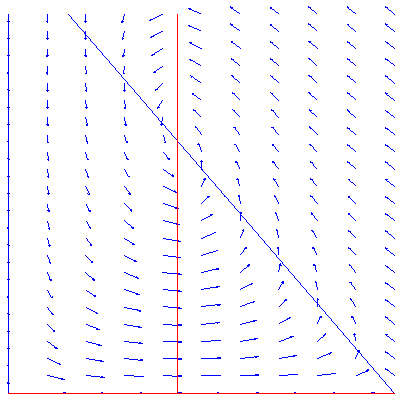
In the next picture the vectors are normalized that they all have the same length. This is called the directional field for F.
| > |
![display(dirfield(F, 1, 2.2), implicitplot([P[1] = 0, VectorCalculus:-`+`(P[1], VectorCalculus:-`*`(VectorCalculus:-`*`(.5, `/`(1.3)), P[2])) = 1, P[1] = VectorCalculus:-`*`(.7, `/`(1.6)), P[2] = 0], P...](images/lotka_volterra_177.gif)
![display(dirfield(F, 1, 2.2), implicitplot([P[1] = 0, VectorCalculus:-`+`(P[1], VectorCalculus:-`*`(VectorCalculus:-`*`(.5, `/`(1.3)), P[2])) = 1, P[1] = VectorCalculus:-`*`(.7, `/`(1.6)), P[2] = 0], P...](images/lotka_volterra_178.gif) |
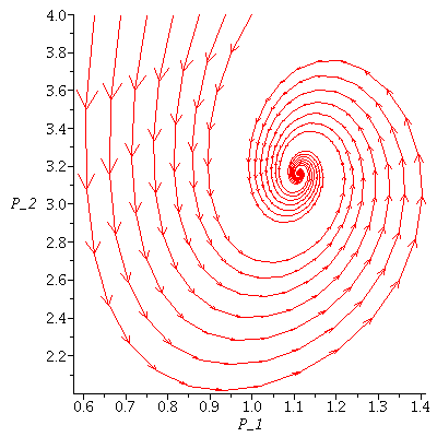
The population orbits through various initial population phases follow the directional field towards the stable equilibrium. (This is called a phase plot of the model.
Here we trace the population orbit through <1,0.1>
| > |
 |
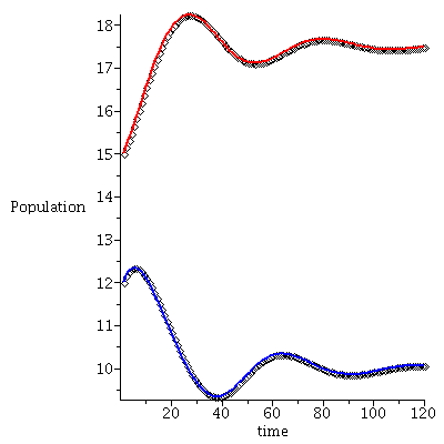
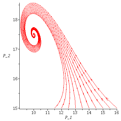
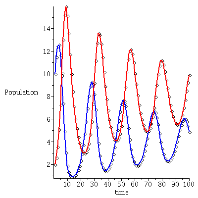
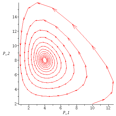
Here is another example of a time plot and a phase plot of a Lotka-Volterra model where the difference in phase between prey and predators is more apparent
| > |
 |

 |
(9) |
| > |
 |
| > |
![display(seq(phasedia(F, P0, 300), P0 = [`<,>`(10, 2)])); 1](images/lotka_volterra_191.gif) |
The equilibria of this model are
| > |
 |
There are two saddle points on the axes and one stable equilibrium in the first quadrant
Paradox of enrichment
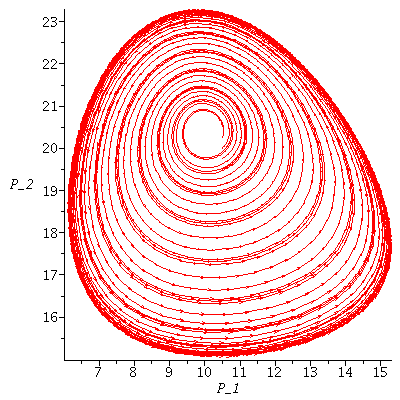
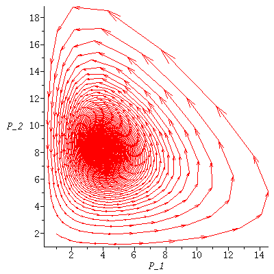
If the carrying capacity of the prey population increases, then the system becomes unstable. (This can be seen as a warning against enrichment of prey populations!) It is unclear if the population orbits in all cases converge to an (infinite) limit cycle.
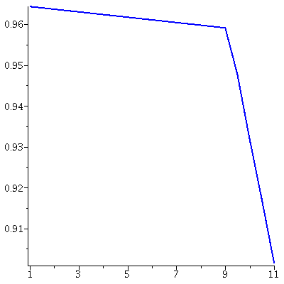
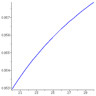
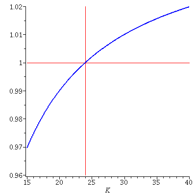
This plot shows the absolute value of the eigenvalues at the co-existence equilibrium for the LV-model LV(K, .5, .05, .2, .05) for K from 15 to 40.
Notice that the co-existence equilibrium is stable for K<24 and unstable for K>24.
| > |
 |
 |
(11) |
| > |
 |
 |
(12) |
When K=23.5 the population orbit through <1,2> converges to the co-existence equilibrium but when K=25 the orbit never reaches the equilibrium.
| > |
 |
| > |
 |
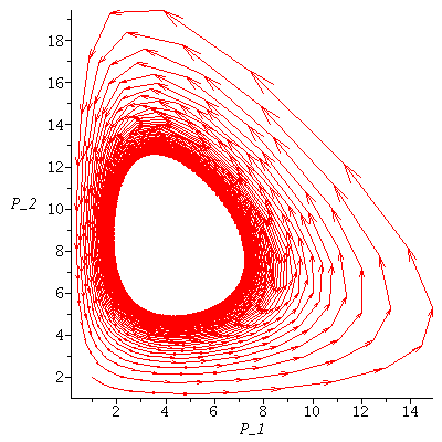
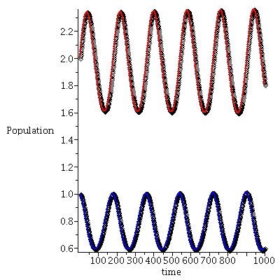
It might be that there exists a limit cycle when the equilibrium is unstable. (When the equilibrium is stable, this limit cycle degenerates to a point.) If this is true, there is really no "paradox of enrichment".
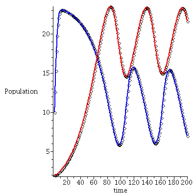
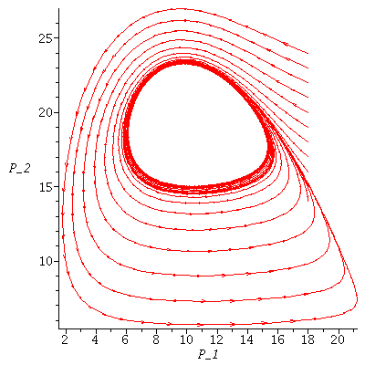
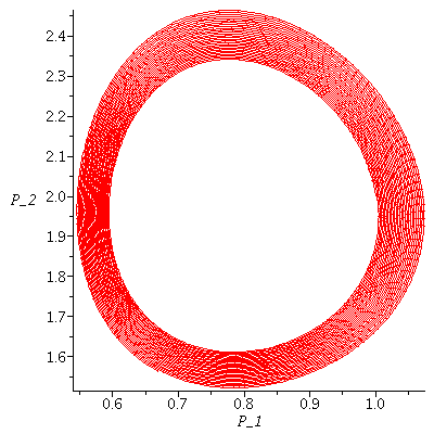
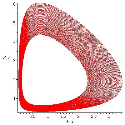
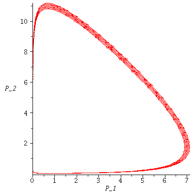
Here is another example of Lotka-Volterra model with an unstable co-existence equilibrium. Is there an infinite limit cycle or is it an artifact of the computer?
| > |
 |

 |
(13) |
| > |
 |
 |
(14) |
| > |
 |
| > |
 |
| > |
 |
| > |
 |
| > |
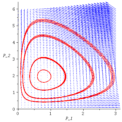
![display([growth(F, 3.0, 6.0), seq(phasedia(F, P0, 1000), P0 = [`<,>`(1, 2), `<,>`(1, 1.2), `<,>`(.4, .5), `<,>`(1.5, .8)])]); 1](images/lotka_volterra_226.gif)
![display([growth(F, 3.0, 6.0), seq(phasedia(F, P0, 1000), P0 = [`<,>`(1, 2), `<,>`(1, 1.2), `<,>`(.4, .5), `<,>`(1.5, .8)])]); 1](images/lotka_volterra_227.gif) |
In this example, it looks as if there are many limit cycles.
The equilibria of this model are
| > |
 |
There are two saddle points on the axes and one unstable equilibrium in the first quadrant.
Let P^* be the co-existence equilibrium in the first quadrant.
These example indicate that
- if P^* is stable then the population orbits will spiral towards P^*
- if P^* is unstable then the population orbits circle, but never reaches, P^*
Avariant of the LV-model with an upper limit for the catch of the predators
| > |
 `(`+`(`*`(`+`(1, `*`(r, `*`(`+`(1, `-`(`/`(`*`(P[1]), `*`(K))))))..." align="center" border="0"> `(`+`(`*`(`+`(1, `*`(r, `*`(`+`(1, `-`(`/`(`*`(P[1]), `*`(K))))))..." align="center" border="0">
 `(`+`(`*`(`+`(1, `*`(r, `*`(`+`(1, `-`(`/`(`*`(P[1]), `*`(K))))))..." align="center" border="0"> `(`+`(`*`(`+`(1, `*`(r, `*`(`+`(1, `-`(`/`(`*`(P[1]), `*`(K))))))..." align="center" border="0">
 `(`+`(`*`(`+`(1, `*`(r, `*`(`+`(1, `-`(`/`(`*`(P[1]), `*`(K))))))..." align="center" border="0"> `(`+`(`*`(`+`(1, `*`(r, `*`(`+`(1, `-`(`/`(`*`(P[1]), `*`(K))))))..." align="center" border="0">
 `(`+`(`*`(`+`(1, `*`(r, `*`(`+`(1, `-`(`/`(`*`(P[1]), `*`(K))))))..." align="center" border="0"> `(`+`(`*`(`+`(1, `*`(r, `*`(`+`(1, `-`(`/`(`*`(P[1]), `*`(K))))))..." align="center" border="0">
 `(`+`(`*`(`+`(1, `*`(r, `*`(`+`(1, `-`(`/`(`*`(P[1]), `*`(K))))))..." align="center" border="0"> `(`+`(`*`(`+`(1, `*`(r, `*`(`+`(1, `-`(`/`(`*`(P[1]), `*`(K))))))..." align="center" border="0">
 `(`+`(`*`(`+`(1, `*`(r, `*`(`+`(1, `-`(`/`(`*`(P[1]), `*`(K))))))..." align="center" border="0"> `(`+`(`*`(`+`(1, `*`(r, `*`(`+`(1, `-`(`/`(`*`(P[1]), `*`(K))))))..." align="center" border="0"> |
| > |
 |
Here is a concrete example.
| > |
 |
| > |
 |
| > |
 |
| > |
![display([seq(phasedia(F, P0, 500), P0 = {seq(`<,>`(VectorCalculus:-`+`(11, VectorCalculus:-`*`(.5, k)), 15), k = 1 .. 10)})]); 1](images/lotka_volterra_277.gif) |
| > |
![display([seq(phasedia(F, P0, 200), P0 = {seq(`<,>`(8, VectorCalculus:-`*`(.5, k)), k = 1 .. 32)})]); 1](images/lotka_volterra_279.gif) |
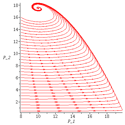
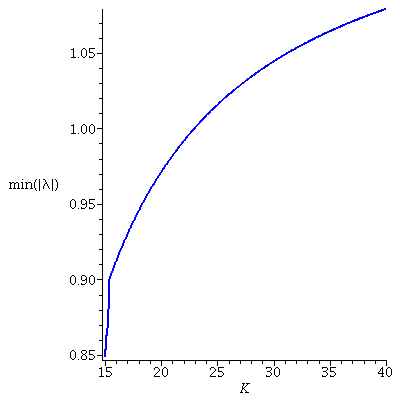
Again, we see that the co-existence equilibrium becomes unstable when K is large (paradox of enrichment)
| > |
![pointplot({seq([K, equi2p(LV2(K, .5, 0.5e-1, .2, 0.7e-1, 4))], K = {seq(VectorCalculus:-`+`(15, VectorCalculus:-`*`(0.5e-1, k)), k = 0 .. 500)})}, connect = true, thickness = 2, color = blue, labels =...](images/lotka_volterra_281.gif)
![pointplot({seq([K, equi2p(LV2(K, .5, 0.5e-1, .2, 0.7e-1, 4))], K = {seq(VectorCalculus:-`+`(15, VectorCalculus:-`*`(0.5e-1, k)), k = 0 .. 500)})}, connect = true, thickness = 2, color = blue, labels =...](images/lotka_volterra_282.gif) |
The co-existence equilibrium is stable when K<22 and unstable when K>23
| > |
 |
 |
(18) |
| > |
 |
 |
(19) |
Here is an example where the co-existence equilibrium is unstable
| > |
 |
| > |
 |
| > |
 |
| > |
![display([seq(phasedia(F, `<,>`(18, VectorCalculus:-`+`(12, k)), 200), k = 2 .. 12)]); 1](images/lotka_volterra_299.gif) |
| > |
![display([seq(phasedia(F, `<,>`(10.5, VectorCalculus:-`+`(20, VectorCalculus:-`*`(.25, k))), 500), k = VectorCalculus:-`-`(2) .. 2)]); 1](images/lotka_volterra_301.gif) |
Another variant of the LV-model
| > |
 `(`+`(`*`(evalf(`+`(1, `*`(r, `*`(`+`(1, `-`(`/`(`*`(P[1]), `*`(K)))..." align="center" border="0"> `(`+`(`*`(evalf(`+`(1, `*`(r, `*`(`+`(1, `-`(`/`(`*`(P[1]), `*`(K)))..." align="center" border="0">
 `(`+`(`*`(evalf(`+`(1, `*`(r, `*`(`+`(1, `-`(`/`(`*`(P[1]), `*`(K)))..." align="center" border="0"> `(`+`(`*`(evalf(`+`(1, `*`(r, `*`(`+`(1, `-`(`/`(`*`(P[1]), `*`(K)))..." align="center" border="0">
 `(`+`(`*`(evalf(`+`(1, `*`(r, `*`(`+`(1, `-`(`/`(`*`(P[1]), `*`(K)))..." align="center" border="0"> `(`+`(`*`(evalf(`+`(1, `*`(r, `*`(`+`(1, `-`(`/`(`*`(P[1]), `*`(K)))..." align="center" border="0">
 `(`+`(`*`(evalf(`+`(1, `*`(r, `*`(`+`(1, `-`(`/`(`*`(P[1]), `*`(K)))..." align="center" border="0"> `(`+`(`*`(evalf(`+`(1, `*`(r, `*`(`+`(1, `-`(`/`(`*`(P[1]), `*`(K)))..." align="center" border="0">
 `(`+`(`*`(evalf(`+`(1, `*`(r, `*`(`+`(1, `-`(`/`(`*`(P[1]), `*`(K)))..." align="center" border="0"> `(`+`(`*`(evalf(`+`(1, `*`(r, `*`(`+`(1, `-`(`/`(`*`(P[1]), `*`(K)))..." align="center" border="0">
 `(`+`(`*`(evalf(`+`(1, `*`(r, `*`(`+`(1, `-`(`/`(`*`(P[1]), `*`(K)))..." align="center" border="0"> `(`+`(`*`(evalf(`+`(1, `*`(r, `*`(`+`(1, `-`(`/`(`*`(P[1]), `*`(K)))..." align="center" border="0"> |
Example 1
| > |
 |
| > |
![solve({F(P)[1] = P[1], F(P)[2] = P[2]}, [P[1], P[2]]); 1](images/lotka_volterra_310.gif) |
![[[P[1] = 0., P[2] = 0.], [P[1] = 10., P[2] = 0.], [P[1] = 8.429319372, P[2] = 52.20251638]]](images/lotka_volterra_311.gif) |
(21) |
| > |
 |
| > |
 |
 |
(22) |
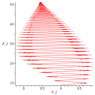
The paradox of enrichment seems to have vanished!
| > |
![pointplot({seq([K, equi2p(LV3(K, 2.3, 0.5e-1, 0.7e-1, 0.6e-1))], K = {seq(VectorCalculus:-`+`(1, VectorCalculus:-`*`(.5, k)), k = 0 .. 20)})}, connect = true, thickness = 2, color = blue); 1](images/lotka_volterra_316.gif)
![pointplot({seq([K, equi2p(LV3(K, 2.3, 0.5e-1, 0.7e-1, 0.6e-1))], K = {seq(VectorCalculus:-`+`(1, VectorCalculus:-`*`(.5, k)), k = 0 .. 20)})}, connect = true, thickness = 2, color = blue); 1](images/lotka_volterra_317.gif) |
Example 2
| > |
 |
| > |
 |
| > |
![solve({`>`(P[1], 0), `>`(P[2], 0), F(P)[1] = P[1], F(P)[2] = P[2]}, [P[1], P[2]]); 1](images/lotka_volterra_322.gif) |
![[[P[1] = 1.111111110, P[2] = 3.160493827]]](images/lotka_volterra_323.gif) |
(23) |
| > |
 |
 |
(24) |
| > |
![pointplot({seq([K, equi2p(LV3(K, .5, .25, .25, .4))], K = {seq(VectorCalculus:-`+`(20, VectorCalculus:-`*`(.5, k)), k = 0 .. 20)})}, connect = true, thickness = 2, color = blue); 1](images/lotka_volterra_326.gif)
![pointplot({seq([K, equi2p(LV3(K, .5, .25, .25, .4))], K = {seq(VectorCalculus:-`+`(20, VectorCalculus:-`*`(.5, k)), k = 0 .. 20)})}, connect = true, thickness = 2, color = blue); 1](images/lotka_volterra_327.gif) |
| > |
 |
 |
(25) |
, Vector[column](%id = 139259608), Vector[column](%id = 138981316)](images/lotka_volterra_153.gif)
, Vector[column](%id = 141190644), Vector[column](%id = 140691284)](images/lotka_volterra_155.gif)

, Vector[column](%id = 137676280), Vector[column](%id = 141403084)](images/lotka_volterra_247.gif)
, Vector[column](%id = 141454516), Vector[column](%id = 141631696)](images/lotka_volterra_257.gif)
