The Ricker Model
If you click on !!! (the menu bar at the top) maple will execute all commands.
You can also enter each command as you go along reading this document. You may enter your own commands at any time and place in this document.
| > |
 |
The projection function for the Ricker model
| > |

 |
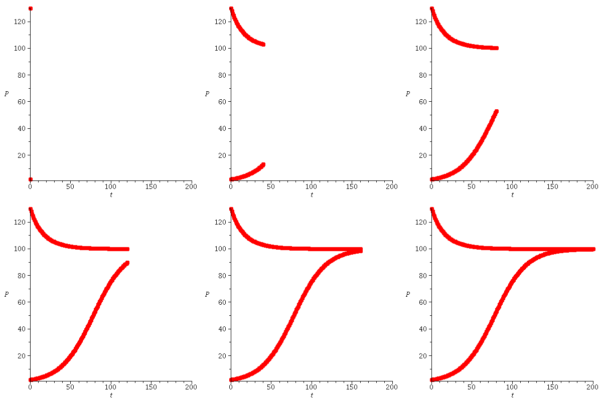
and the population dynamics
| > |
![display([dynplotfilm(ricker(0.5e-1, 100), 2, 200), dynplotfilm(ricker(0.5e-1, 100), 130, 200)]); 1](images/ricker_111.gif) |
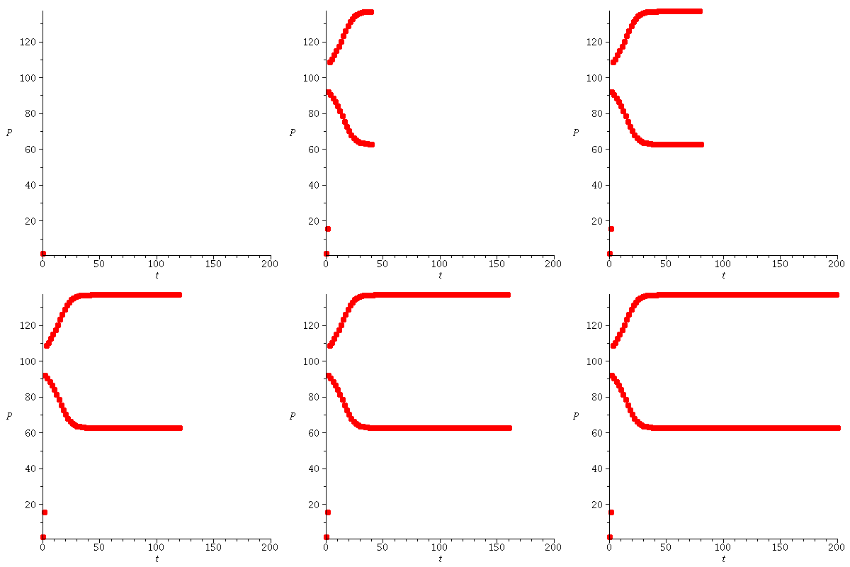
The population dynamics for a higher value of r
| > |
 |
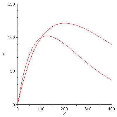
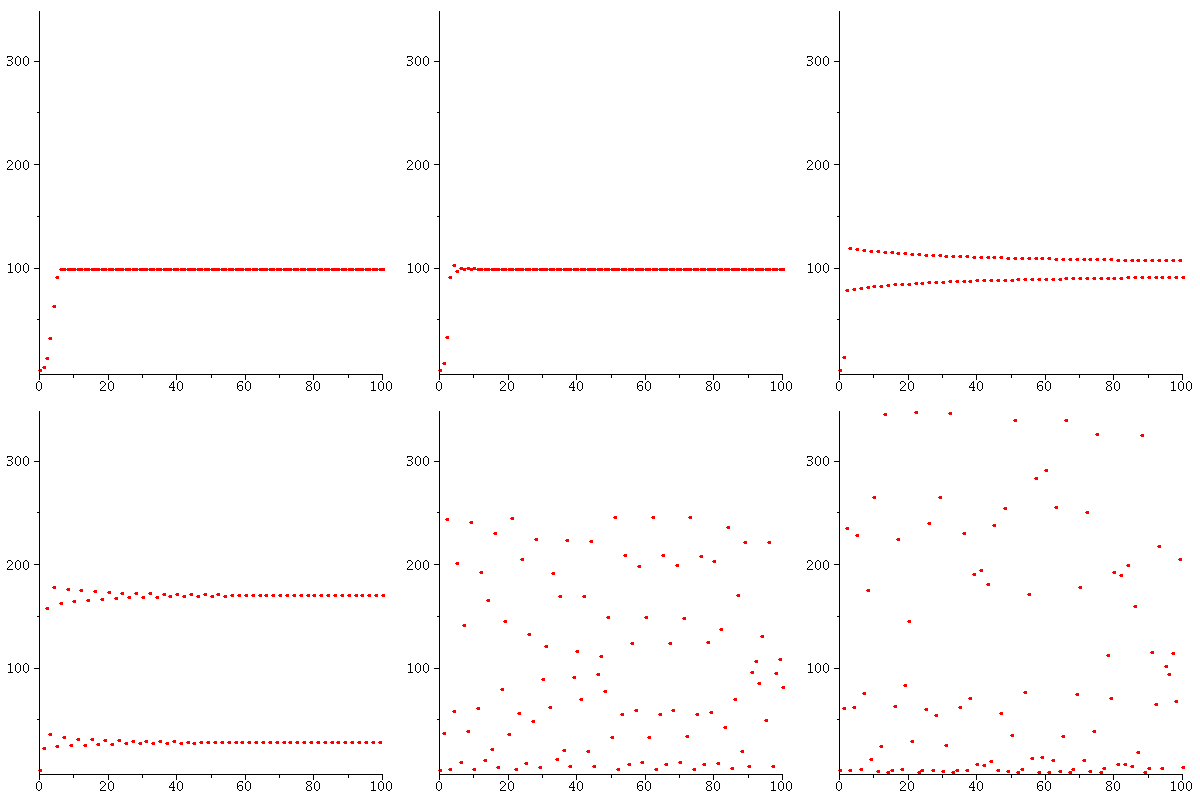
Ricker models with various values of the parameter r
| > |
 |
There are two equilibria when r<2.
When r<2, 0 is an unstable equilibrium, and the carrying capacity K is a stable equilibrium. We can see this by computing
| > |
 |
![[0., 6.049647464], [0., 6.049647464]](images/ricker_118.gif) |
(1) |
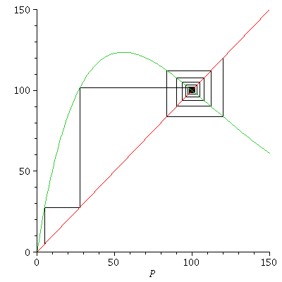
or by looking at a cobweb diagram
| > |
 |
where we see that all population orbits converge to the carrying capacity
| > |
![seq(iterate(ricker(1.8, 100), P0, 200), P0 = [1, 5, 6, 150, 250]); 1](images/ricker_122.gif) |
 |
(2) |
Let us now consider the case where r>2.
We look for a stable 2-cycle for r=
| > |
 |
 |
(3) |
which is shown in frame 25 above.
| > |
 |
 |
(4) |
We first try to solve the equation FF(P)=P,
| > |
 |
![[0., 90.01713129], [0., 90.01713129]](images/ricker_129.gif) |
(5) |
Well, it seems to be beyond maple's powers to solve the equation FF(P)=P!
Maybe we can solve graphically
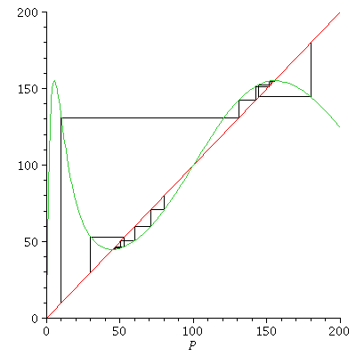
Let us look at some cobweb diagrams for F^2
| > |

 |
It looks as if there are stable 2-cycles near 50 and 150. We approximate this 2-cycle by orbits:
| > |
![seq(iterate(proc (P) options operator, arrow; F(F(P)) end proc, P0, 300), P0 = [10, 30, 80, 180]); 1](images/ricker_133.gif) |
 |
(6) |
and see that we really arrived at a 2-cycle
| > |
![orbit(F, %[1], 6); 1](images/ricker_135.gif) |
 |
(7) |
We check if it is stable
| > |
 |
 |
(8) |
| > |
 |
 |
(9) |
Yes, the 2-cycle (44.88, 155.11) is stable.
| > |
, P0, 500)), P0 = [10, 20, 30, 45, 50])}; 1](images/ricker_141.gif) |
 |
(10) |
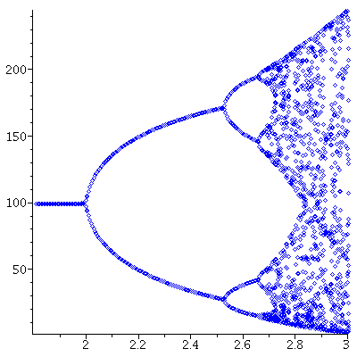
The stable orbits of the Ricker model can be illutstrated in the bifurcation diagram
| > |
![pointplot([seq(seq([`+`(1.8, `*`(0.5e-2, `*`(i))), orbit(ricker(`+`(1.8, `*`(0.5e-2, `*`(i))), 100), 80, 250)[j]], j = 230 .. 250), i = 1 .. 240)], style = point, color = blue); 1](images/ricker_143.gif)
![pointplot([seq(seq([`+`(1.8, `*`(0.5e-2, `*`(i))), orbit(ricker(`+`(1.8, `*`(0.5e-2, `*`(i))), 100), 80, 250)[j]], j = 230 .. 250), i = 1 .. 240)], style = point, color = blue); 1](images/ricker_144.gif) |
![]()
